|
|
|
|
|
|
In our model for RNA secondary structure formation we assume that each of the candidate helices (see definition in the main text) may exist in two states. A helix can be completely zipped, or it can be completely decayed. This effectively targets the time scale of RNA secondary structure transitions that is of order of 10-3sec. The following schema is used to estimate the effective transition constants between zipped and decayed states:
· Spontaneous decay of a helix occurs as a set of consecutive unzipings of the terminal nucleotide
pairs. It can be thought of as a branching Markov process (Figure 1).
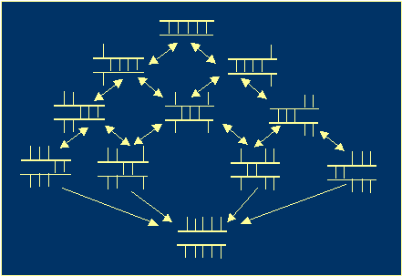 |
Figure 1. A helix decay process. |
· Formation of a new helix occurs in two steps: formation of the
loop and zipping of the helix. To determine the kinetic constants, we use
the transition state theory, which is often used in chemical kinetics
(Figure 2).
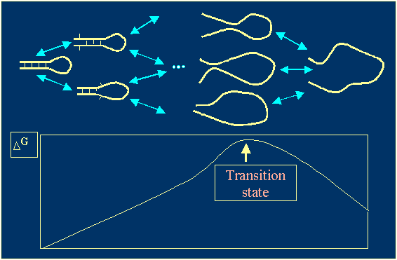 |
Figure 2. Transition states of a helix formation process. |
We calculate the kinetic constants based on the following observations:
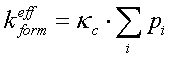
where ![]() is probability
of i-th transition state and k
is probability
of i-th transition state and k![]() is an elementary event constant. Suppose that all the transition states probabilities
are equal. Thus,
is an elementary event constant. Suppose that all the transition states probabilities
are equal. Thus,
![]()
here ![]() denotes the stacking pairs number in the helix. The probability to form a loop
relates to the entropy loss as
denotes the stacking pairs number in the helix. The probability to form a loop
relates to the entropy loss as
![]()
hence
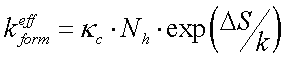
As far as the loop free energy is purely entropic,
![]()
Finally for formation constant:
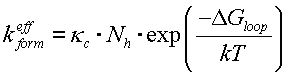 |
(1) |
We can obtain the helix decay constant from (1) via the Van't Hoff's law:
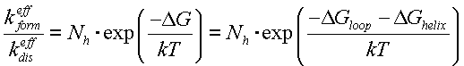
Finally, we get the decay constant:
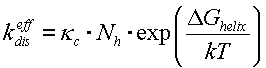 |
(2) |
One can obtain the same formulae considering helix decay as a
branching Markov process (Figure 1). Thus the physical sense of the constant
![]() can be clarified.
Thise constant is the constant of the last nucleotide pair locking on the helix
growths. Its value is estimated as 1.e+6 .. 1.e+8 (Porske, 1974). Here is a
table of characteristic times for some events given .
can be clarified.
Thise constant is the constant of the last nucleotide pair locking on the helix
growths. Its value is estimated as 1.e+6 .. 1.e+8 (Porske, 1974). Here is a
table of characteristic times for some events given .
|
Transition
|
time
|
| A formation of a 5-nucleotide helix with a hairpin loop of 6 nucleotides (i.e. the most favorable helix) | 2.e-4 |
| A spontaneous decay of a helix containing 5 A-U nucleotide pairs | 8.e-4 |
| A spontaneous decay of a helix containing 5 G-C nucleotide pairs | 1.4e+4 |
| A spontaneous decay of a helix containing 8 G-C nucleotide pairs | 4.7e+10=1500 years!!! |
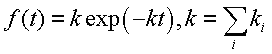
The RNA secondary structure formation can be represented as a Markov process. The states of the process are the secondary structures, the transitions are a new helix formation or an existing helix decay. As far as the transitions are uniform (i.e. at any time, their probabilities do not depend on the time count start), ordinary (i.e. only one transition is possible at any time), and history-independent (transitions probabilities depend only on current state rather than on pre-history), the transition time is a random, exponentially-distributed random value
![]()
The modeling process is the following.
1. We enumerate all the potential (candidate) helices with lifetime that exceed
a given threshold.
2. We initiate the process with a trivial structure with no helices.
3. For the current state (structure), we form a complete list of potential transitions
with their probabilities from all existing helices decay, all possible helices
(i.e. that do not contradict with any of existing helices) formation, and the
chain elongation.
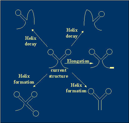 |
Figure 3 The definition of possible transitions. |
4. The kinetic constants are calculated for these transitions.
5. We choose the transition to execute. A random value drawn uniformly from
the interval wher

and then the number of the transition is defined from
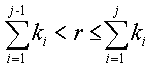
The time between the transition and the pervious one is drawn from the exponential
distribution
5. The chosen transition is executed and the experiment time is incremented
by .
6. If the current time is still less than a pre-given value of the overall
experiment time, return to 3.
7. If the times of runs we made is less than a pre-given number N, return
to 2.
The result of the algorithm work is kinetic ensemble of secondary RNA structures,
i.e. a set of secondary structures with their time-dependent probabilities.
The relative precision of the probabilities evaluation can be estimated by
as ![]() . To include
the RNA molecule synthesis, it is enough to start from zero length chain on
step 2 and to add the chain elongation by 1 nucleotide as a possible transition.
The constant for this transition is usually .
. To include
the RNA molecule synthesis, it is enough to start from zero length chain on
step 2 and to add the chain elongation by 1 nucleotide as a possible transition.
The constant for this transition is usually .
![]()
Virtually, the helices are not independent. They can overlap. Let's consider
a classification of mutual positions of two candidate helices (Figure 4).
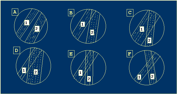 |
Figure 4 Possible mutual positions of two candidate helices. |
· Complete compatibility (A). The second helix can form without the
first helix decay.
· Partial compatibility (B). The helix 2 can be freely initiated, but
the there are helix positions overlap, and a sliding loop is formed between
two helices.
· One of the strands of helix 2 is located inside a strand of helix 1
(C). It is necessary to untwist helix 1 partially to initiate helix 2. After
the initiation, the helix 2 will be supplanted by helix 1. If helix 2 exists,
helix 1 can be freely initiated and then it will supplant helix 2.
· It is necessary to untwist helix 1 partially to initiate helix 2 (D).
After it, 1 will supplant 2 and nothing happens.
· The helix 2 can be initiated freely (E). Then, helix 2 supplants helix
1 and there is no helix 1 in the final structure.
· A pseudo-knot (F). In this case, to initiate helix 2 it is necessary
either to overcome the pseudo-knot formation energetic threshold or to decay
helix 1 completely.
Another characteristic of the refined model is that we do not treat helix decay
as a sufficient event, because a new helix can form (possibly, the same) after
decay. The process of new helix formation given that it is hampered by other
helices can be represented as a set of elementary events.
| decay of all hampering helices | the free energy increases |
| new helix initiation | the free energy increases |
| the helix formation completing | the free energy decreases |
There are several ways to form the new helix, though the final structure is
the same for all of them. All the events except the last increase the free energy,
so we can evaluate the transition constant as
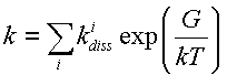 |
(3) |
here G is the transition free energy, is constant of a reverse from the final state to the to one of the pre-final (threshold) states, i.
Let's verify the formula. A threshold transition occurs, thus the flux is summarized over all fluxes from all the pre-final states,
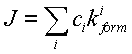 ,
,
where![]() is probability of i-th pre-final state,
is probability of i-th pre-final state, ![]() is the constant of the transition from the state to the final one. The flux
is relatively small, so we can suppose that is close to the balanced value
is the constant of the transition from the state to the final one. The flux
is relatively small, so we can suppose that is close to the balanced value
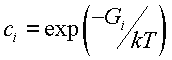
where ![]() is energy of i-th pre-final state relative to the final state.
The Van't Hoff's law requires:
is energy of i-th pre-final state relative to the final state.
The Van't Hoff's law requires:
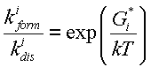 ,
,
whre in ![]() energy
of -th pre-final state relative to the final state. Thus, we obtain the formula
(3).
energy
of -th pre-final state relative to the final state. Thus, we obtain the formula
(3).
Porshke D. (1974). A direct measurement of the unzippering rate of a nucleic
acid double helix. Biophys.Chem.. 2: 97-101